Busting Myths about EBSD Pattern Matching

14^th July 2023 | Author: Pat Trimby

When I take a look at recent publications and conference presentations involving developments in the field of electron backscatter diffraction (EBSD), then it is clear that the use of simulated patterns and pattern matching techniques are becoming increasingly popular. Indeed, only last year I wrote a blog that suggested that pattern matching represented a paradigm shift for EBSD – you can read that here. A year later and I feel that my assessment was spot on – we are using pattern matching increasingly frequently and to solve many different problems, including:

• Indexing poor-quality diffraction patterns (e.g. from highly deformed structures)
• Improving angular precision (e.g. to resolve orientation changes associated with individual dislocations)
• Discriminating between phases that have similar structures
• Correcting indexing measurement errors, including those attributed to pseudosymmetry effects
• Resolving the subtle changes in EBSD patterns caused by different polarities / inversion domains

It’s great that more and more of our customers are getting access to the unique pattern matching tools available in AZtecCrystal MapSweeper, but sometimes it is wise to keep our excitement in check, at least just a little bit. In this blog, I want to address some of the myths associated with EBSD pattern matching techniques and, hopefully, to provide some useful pointers to those of you who are already taking advantage of MapSweeper’s capabilities to improve your materials characterisation.

1. I don’t need to worry about indexing results at the SEM

Ever since we launched our first Symmetry CMOS-based detector in 2017, one of the strengths of EBSD has been the short time it takes to characterise standard materials (e.g. steels, alloys etc.). Routinely, we now analyse at speeds exceeding 4000 indexed patterns per second (pps); this means that we can characterise the grain size and texture to international standards in just a few minutes. This is fantastic progress compared to a decade or more ago!

A lot of the properties that we measure using EBSD, such as the texture, grain size and phase fraction, are instantaneously attained. We get our answers at the microscope without need for any subsequent data processing. So why would we throw these data away and go through the process of reanalysing stored patterns to reproduce the same results? It makes little sense. Therefore, if you have a sample that is relatively easy to characterise and you are focused on measuring routine microstructural parameters, then the live indexing using the Hough-transform method will deliver all the information you need both quickly and effectively.

Even if you have a difficult sample – say one that is highly deformed or has lots of low symmetry phases (such as in a typical rock sample or ceramic coating), then focusing on getting good results at the microscope will save lots of time if you do proceed with a reanalysis using pattern matching. This is because many of the most powerful tools in MapSweeper use a hybrid pattern matching approach; the original phase and orientation result at each point informs the simulated template generation, so that the software does not need to evaluate (at significant time expense) all possible phases and orientations. The better your initial data from the live indexing process at the SEM, the more effective your subsequent reanalysis in MapSweeper will be.

2. There’s no need for careful sample preparation

When I first introduced MapSweeper to a colleague, their initial reaction was to ask “does this mean that we don’t need to worry about the sample preparation?”. The answer is an emphatic “No!”.

It is true that pattern matching allows us to index very poor-quality patterns. This is great news for the analysis of highly-deformed, beam-sensitive or nanostructured materials, but it does not mean that we should take shortcuts in our sample preparation procedure. In fact, if anything, pattern matching will highlight the deficiencies in our sample preparation even more, and it becomes clear that, instead of measuring the key microstructural properties of the sample, we end up measuring damage and artefacts caused by the poor preparation. You can see this in the following maps taken from a recent analysis of a garnet grain in a metamorphic rock sample. There is no discernible orientation variation in the inverse pole figure map, although the band contrast map does indicate that there might be one or two surface scratches. However, after reanalysing with MapSweeper, we see the clear impact of scratches on the normalised cross correlation coefficient; given that this analysis was focusing on small orientation changes within large garnet grains, the data were severely compromised by the poor sample preparation.

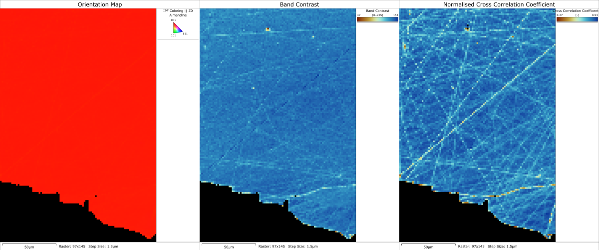
Sample preparation damage in a garnet grain. Left – inverse pole figure orientation map. Centre – band contrast pattern quality map from conventional Hough-based indexing. Right – normalised cross correlation coefficient map following reanalysis using pattern matching.

So, when using pattern matching methods, sample preparation becomes even more important than it was for conventional EBSD methods, not less.

3. You should store EBSD patterns with every dataset

This is a slightly trickier topic to address. Since we started developing MapSweeper, I have been reprocessing many old datasets from my previous job in academia and have been able to extract much better information from various challenging samples. So, in retrospect, I am delighted that I had the foresight to store the patterns more than 10 years ago. However, that does not mean that this should be our routine approach.

If you are interested in routine characterisation of a series of samples, then there would be no need to save the patterns. For example, you have a number of heat-treated steels and you need to measure the effect of the heat treatment on the phase fraction, texture and grain size, then it is unlikely that you would benefit from reprocessing the data using pattern matching methods. Therefore, there would be no sense in storing all of the patterns. However, if you have a more open-ended research target, for example you want to investigate the wider impact of the heat treatment on the microstructure, then pattern storage would be more sensible – potentially, in the future, you may want to improve the angular precision of the measurements, or perhaps there would be additional phases present that you did not expect, or maybe there will be pattern matching methods available in the future that would provide further insight into the material’s properties.

However, a practical consideration of the volume of data is necessary. Routinely, we are saving 10s GB of data per hour at the microscope. This poses specific challenges on disk space, data transfer and subsequent storage, and a lot of our IT infrastructure has not been developed with this in mind. Therefore, we may have to temper our enthusiasm to reprocess every dataset using pattern matching, focusing on those investigations where we know that our research will benefit from the additional quality of data that pattern matching provides.

4. Pattern Matching techniques can index everything

Ever since dictionary indexing was first demonstrated, one of the appeals of pattern matching methods has been its ability to index even the poorest quality pattern. It makes no sense to use this technology to cut corners on your experimental set up (for example, don’t compromise on pattern quality just because you know that you can index noisy patterns using pattern matching), but if you have a particularly challenging sample, then pattern matching can make a dramatic difference to your indexing rate and overall data quality.

However, it’s worth understanding that pattern matching methods will manage to “index” every single pattern. There will always be a simulated pattern template that matches an experimental pattern best, regardless of how good that diffraction pattern is. We can take this to the extreme and see what happens when we try and use pattern matching to index something that is not a diffraction pattern. Like a photo of an elephant!

The answer, as you can see below, is that we can indeed index the elephant quite well (with a Ni structure, no less):

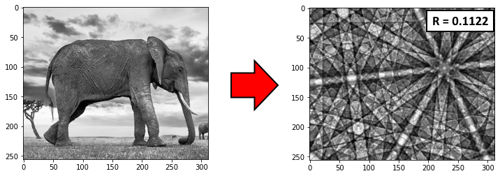
Indexing an elephant as Ni – the best fitting simulated pattern matches with a normalised cross correlation coefficient (R) of 0.1122.

This is where we need to be careful – as we can always get a solution, we will be able to get indexed solutions at points where we don’t even have any diffraction (e.g. from voids, epoxy mounts, dust particles etc.). So, this makes it very important that we have a robust metric for measuring the image similarity between the experimental and simulated patterns. In MapSweeper, we use the normalised cross correlation (NCC) coefficient, whereas other pattern matching methods tend to use the normalised dot product (NDP) approach.

Note that, compared to the NCC, the NDP involves neither the removal of the mean from the image nor a normalization according to the image intensity. These make the NDP much less useful as an image similarity measure when the images that are being compared vary in either intensity or mean level. Given that most EBSD patterns will have variations in these values (e.g. as the beam scans across different phases, voids, surface topography or, in the case of TKD, different sample thicknesses), then it is clear that the NCC will be a significantly more robust metric than the NDP. If we return to the elephant, then this becomes apparent as we change the image intensity or mean – the NCC value remains constant (until we try to index the elephant with an image that is just noise), whereas the NDP varies significantly as the image levels change. So for the NDP, where would you set the threshold value in order to reject false solutions?

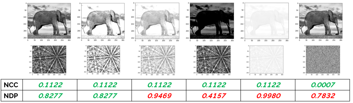
Variations in image similarity measures (normalised cross correlation – NCC, normalised dot product – NDP) between a picture of an elephant and the best fitting simulated Ni pattern, with varying image intensities and mean.

So the message here is twofold:

1. We need to set a sensible threshold value for our image similarity so that we don’t accept false positive solutions
2. The normalised cross correlation coefficient is a far more robust method of measuring the pattern similarities than the normalised dot product

Next time you try and analyse a difficult sample, ensure that you set the NCC coefficient threshold to a sensible value (e.g. use the default of 0.15) and then you can be confident that you are collecting great data without accepting invalid solutions.

If you are interested in learning more about MapSweeper, click here or contact us to receive a copy of the new MapSweeper brochure.

About the Author